[논문 리뷰] SRCNN의 Hyperparameter에 대해 알아보자.

논문을 바탕으로 하여 SRCNN의 Hyperparameter에 대해 알아보고, 왜 해당 값으로 정해졌는지에 대해 분석해보자.

$$F_{1}(Y) = max(0, W_{1}*Y+B_{1})$$ 

 

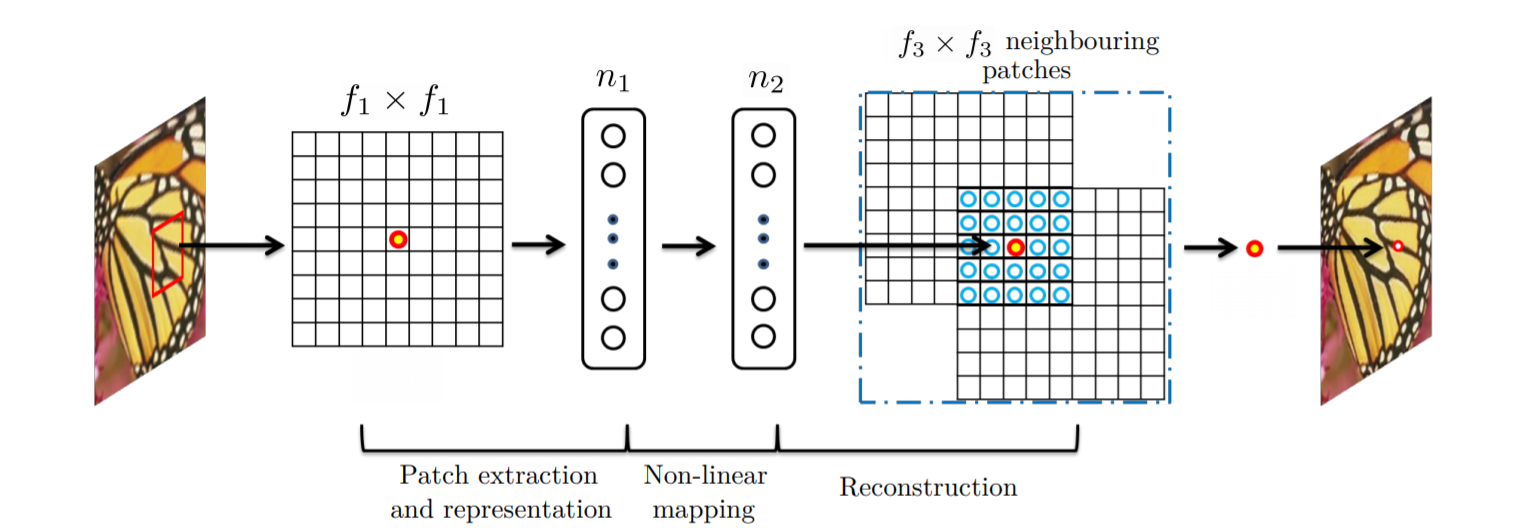
W1, B1 represent the filters and biases respectivley. W1 corresponds to n1 filters of support c*f1*f1, where c is the number of channels in the input image, f1 is the spatial size of a filter. Intuitively, W1 applies n1 convolutions on the image, and each convolution has a kernel size c*f1*f1. The output is composed of n1 feature maps. B1 is an n1-dimensional vector, whose each element is associated with a filter. Then apply the ReLU on the filter responses. This first layer extract an n1-dimensional feature for each patch. 

W1, B1은 각각 filters and biases을 나타낸다. W1은 c*f1*f1를 support하는 n1개의 필터에 해당하며, 여기서 c는 입력 이미지의 채널 수, f1은 필터의 공간 크기이다. 직관적으로 W1은 이미지에 n1 컨볼루션(convolution)을 적용하고 각 컨볼루션은 c*f1*f1 크기의 커널을 가진다. 출력은 n1 피쳐 맵으로 구성된다. B1은 n1차원 벡터이며, 각 원소는 필터와 연관되어 있다. 그런 다음 필터 적용 결과에 ReLU를 적용합니다. 이 첫 번째 레이어는 각 패치에 대해 n1차원 기능을 추출한다.

 

 

$$F_{2}*(Y) = max(0, W_{2}*F_{1}(Y)+B_{2})$$

 

Map each of n1-dimensional vectors into an n2-dimensional one. This is equivalent to applying n2 filters wich have a trivial spatial support 1*1. This interpretation is only valid for 1*1 filters. W2 contains n2 filters of size n1*f2*f2, and B2 is n2-dimensional. Each of the output n2-dimensional vecotrs is conceptually a representation of high-resolution patch that will be used for reconstruction.

 

각 n1차원 벡터를 n2차원 벡터로 매핑합니다. 이는 1*1인 n2 필터를 적용하는 것과 같다. 이 해석은 1*1 필터에만 유효합니다. W2에는 n1*f2*f2 크기의 n2 필터가 포함되어 있으며, B2는 n2차원 필터이다. 출력 n2차원 벡터 각각은 개념적으로 재구성에 사용될 고해상도 패치의 표현이다.

 

$$F(Y) = W_{3} * F_{2}(Y) + B_{3}.$$

 

Define a convolutional layer to produce the final high-resolution image. W3 corresponds to c filters of a size n2*f3*f3, and B3 is a c-dimensional vector. If the representations of the high-resolution patches are in the image domain, we expect that the filters act like an averaging filter. if the representations of the high-resolution patches are in some other domains, we expect that W3 behaves like first projectiong the coefficients onto the image domain and then averaging. In either way, W3 is a set of linear filters.

 

최종 고해상도 이미지를 생성하기 위한 컨볼루션 레이어를 정의합니다. W3은 n2*f3*f3 크기의 c 필터에 해당하며, B3는 c차원 벡터이다. 고해상도 패치의 표현이 이미지 도메인에 있는 경우 필터가 평균 필터처럼 동작할 것으로 예상하며, 고해상도 패치의 표현이 일부 다른 도메인에 있는 경우 W3가 먼저 이미지 도메인에 계수를 투영한 다음 평균을 내는 것처럼 동작할 것으로 예상한다. 어느 쪽이든 W3은 선형 필터의 집합이다.

 

Cf. Sparse representation

Sparse representation, 즉 one-hot encoding은 해당 속성이 가질 수 있는 모든 경우의 수를 각각의 독립적인 차원으로 표현한다. 예를 들어, 해당 단어가 ‘강아지’라는 속성을 표현해보자. 우리가 가진 단어가 총 N개라면 이 속성이 가질 수 있는 경우의 수는 총 N개이다. One-hot encoding에서는 이 속성을 표현하기 위해 N차원의 벡터를 만든다. 그리고 ‘강아지’에 해당하는 요소만 1이고 나머지는 모두 0으로 둔다. 이런 식으로 단어가 가질 수 있는 N개의 모든 경우의 수를 표현할 수 있다.

마찬가지 방식으로 품사가 ‘명사’라는 속성을 표현하고 싶다면 품사의 개수만큼의 차원을 갖는 벡터를 만들고, ‘명사’에 해당하는 요소만 1로 두고 나머지는 모두 0으로 둔다. 다른 속성들도 모두 이런 방식으로 표현할 수 있다.

 

SR method, 기저 함수의 차원을 데이터의 차원보다 크게 세팅한 뒤, 대부분의 sparse code의 계수를 0으로 하고 활성화된 계수들의 수를 소수로 제한한다면 좀 더 밀도있는 표현이 가능하다.

훈련 셋으로부터 학습을 통해 최적의 기저(Dictionary)와 표현될 벡터(sparse code)를 선형 연산을 통해 알아내는 것.

 

 

In the sparse-coding-based methods, let us consider that an f1*f1 low-resolution patch is extracted from the input image. Then the sparse coding solver, like Feature-Sign, will first project the patch onto a (low-resolution) dictionary. If the dictionary size is n1, this is equivalent to applying n1 linear filters(f1*f1) on the input image. 

희소 코딩 기반 방법에서는 입력 이미지에서 f1*f1 저해상도 패치를 추출한다고 가정해 보자. 그런 다음 Feature-Sign과 같은 희소 코딩 솔버는 먼저 패치를 (저해상도) 사전에 투영한다. 사전 크기가 n1이면 입력 영상에 n1 선형 필터(f1*f1)를 적용하는 것과 같습니다.

 

The sparse coding solver will then iteratively process the n1 coefficients. The outputs of this solver are n2 coefficients, and usually n2 = n1 in the case of sparse coding. These n2 coefficients are the representation of the high-resolution patch. In this sense, the sparse coding solver behaves as a special case of non-linear mapping operator, whose spatial support is 1x1. 

그런 다음 희소 코딩 솔버는 n1 계수를 반복적으로 처리합니다. 이 솔버의 출력은 n2 계수이며, 일반적으로 희소 코딩의 경우 n2 = n1이다. 이러한 n2 계수는 고해상도 패치를 나타냅니다. 이러한 의미에서 희소 코딩 솔버는 공간 지원이 1x1인 비선형 매핑 연산자의 특수한 경우로 동작한다.

 

If we set f2=1, then our non-linear operator can be considered as a pixel-wise fully-connected layer. It is worth nothing that "the sparse coding solver" in SRCNN refers to the first two layers, but not just the second layer or the activation function.

 

 

The above n2 coefficients are then projected onto another dictionary to produce a high-resolution patch. The overlapping high-resolution patches are then averaged. This is equivalent to linear convolutions on the n2 feature maps. If the high-resolution patches used for reconstruction are of size f3*f3, then the linear filters have an equivalent spatial support of size f3*f3. 

위의 n2 계수는 고해상도 패치를 생성하기 위해 다른 사전에 투영됩니다. 그런 다음 겹치는 고해상도 패치의 평균을 구합니다. 이는 n2 기능 맵의 선형 컨볼 루션과 동일합니다. 재구성에 사용되는 고해상도 패치의 크기가 f3 * f3 인 경우 선형 필터는 f3 * f3 크기와 동등한 공간 지원을 갖습니다.

 

The above discussion shows that the sparse-codingbased SR method can be viewed as a kind of convolutional neural network (with a different non-linear mapping). But not all operations have been considered in the optimization in the sparse-coding-based SR methods. On the contrary, in our convolutional neural network, the low resolution dictionary, high-resolution dictionary, non-linear mapping, together with mean subtraction and averaging, are all involved in the filters to be optimized. So our method optimizes an end-to-end mapping that consists of all operations.

위의 논의는 희소 부호화 기반 SR 방법을 (다른 비선형 매핑으로) 일종의 컨볼루션 신경망으로 볼 수 있음을 보여준다. 그러나 모든 작업이 희소 코딩 기반 SR 방법의 최적화에서 고려된 것은 아니었다. 반대로, 우리의 컨볼루션 신경망에서는 평균 감산 및 평균과 함께 저해상도 사전, 고해상도 사전, 비선형 매핑이 모두 최적화될 필터에 관련되어 있다. 따라서 우리의 방법은 모든 작업으로 구성된 엔드 투 엔드 매핑을 최적화한다.

 

The above analogy can also help us to design hyperparameters. For example, we can set the filter size of the last layer to be smaller than that of the first layer, and thus we rely more on the central part of the highresolution patch (to the extreme, if f3 = 1, we are using the center pixel with no averaging). We can also set n2 < n1 because it is expected to be sparser. A typical and basic setting is f1 = 9, f2 = 1, f3 = 5, n1 = 64, and n2 = 32. On the whole, the estimation of a high resolution pixel utilizes the information of (9 + 5 − 1)2 = 169 pixels. Clearly, the information exploited for reconstruction is comparatively larger than that used in existing external example-based approaches, e.g., using (5+5−1)2 = 81 pixels5. This is one of the reasons why the SRCNN gives superior performance.

 

---

Questions.

 

- 차원을 줄임으로서 불필요한 것들을 줄이는 과정이라고 이해해도 되는 건가요? (n1차원을 n2차원으로 변경하는 과정)

- f2=1로 세팅하므로서 pixel-wise fc-layer로서의 역할을 한다고 했는데, f1*f1*n1 의 feature map에 1*1*n2 (n2 < n1) 필터를 적용함으로서 정확히 어떤 효과를 얻을 수 있는 것인가요? 

- 마지막 레이어의 필터 사이즈를 첫번째 레이어의 필터 사이즈보다 작게 설정하므로서 rely more on the central part of the high-resolution patch할 수 있다고 하였는데, 이 부분이 정확히 어떤 의미이고 어떤 장점을 가지는 것인가요?

- n2 < n1 으로 설정함으로서 sparser 한 효과를 얻을 수 있다고 하였는데, 이 부분은 SR method에서도 나왔듯이 기저함수의 차원을 데이터의 차원보다 늘리고 활성화된 계수의 수를 소수로 제한한다면 밀도있는 표현이 가능하다고 하였는데, 왜 그런 것인지 이해가 잘 안됩니다.